scRNA-seq analysis
In this tutorial, we’ll utilize the 10X PBMCs scRNA-seq dataset to showcase the steps for running SIMBA on scRNA-seq datasets.
[1]:
import os
import simba as si
si.__version__
[1]:
'1.2'
[2]:
workdir = 'result_simba_rnaseq'
si.settings.set_workdir(workdir)
Saving results in: result_simba_rnaseq
[3]:
si.settings.set_figure_params(dpi=80,
                              style='white',
                              fig_size=[5,5],
                              rc={'image.cmap': 'viridis'})
[4]:
# make plots prettier
from matplotlib_inline.backend_inline import set_matplotlib_formats
set_matplotlib_formats('retina')
[ ]:
load example data
[5]:
adata_CG = si.datasets.rna_10xpmbc3k()
Downloading data ...
rna_10xpmbc3k.h5ad: 21.5MB [00:07, 2.75MB/s]
Downloaded to result_simba_rnaseq/data.
[6]:
adata_CG
[6]:
AnnData object with n_obs × n_vars = 2700 × 32738
    obs: 'celltype'
    var: 'gene_ids'
[ ]:
preprocessing
[7]:
si.pp.filter_genes(adata_CG,min_n_cells=3)
Before filtering:
2700 cells, 32738 genes
Filter genes based on min_n_cells
After filtering out low-expressed genes:
2700 cells, 13714 genes
[8]:
si.pp.cal_qc_rna(adata_CG)
[9]:
si.pl.violin(adata_CG,list_obs=['n_counts','n_genes','pct_mt'])
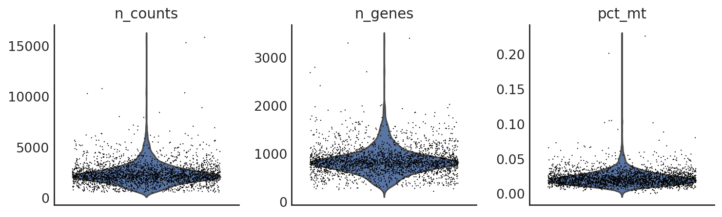
Filter out cells if needed:
si.pp.filter_cells_rna(adata,min_n_genes=100)
[10]:
si.pp.normalize(adata_CG,method='lib_size')
si.pp.log_transform(adata_CG)
[ ]:
Optionally, variable gene selection step can be also performed.
si.pp.select_variable_genes(adata_CG, n_top_genes=2000)
si.pl.variable_genes(adata_CG,show_texts=True)
By encoding only variable genes into the graph, the training procedure can be accelerated. However, the embeddings of non-variable genes will not be acquired.
[ ]:
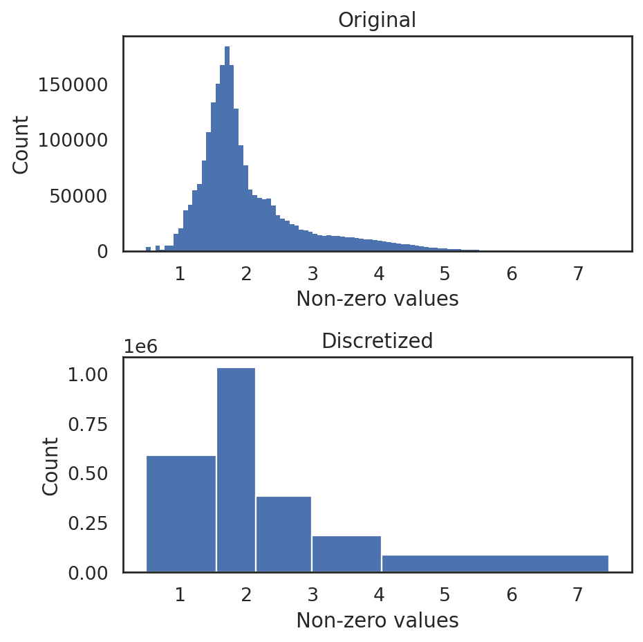
discretize RNA expression
This step groups non-zero gene expression values into distinct levels while preserving the original distribution, enabling recognition of different levels of gene expression during the subsequent training.
[11]:
si.tl.discretize(adata_CG,n_bins=5)
si.pl.discretize(adata_CG,kde=False)
[ ]:
generate a graph for training
Observations and variables within each Anndata object are both represented as nodes (entities).
Anndata objects specified in
list_CG(or other list parameters likelist_adata) will have their nodes automatically matched by comparing their.obs_namesand.var_names.The non-zero values in
.layers['simba'](by default) or.X(if.layers['simba']does not exist) denote edges between nodes.
For gene expression data, by default, different levels of gene expression are encoded by distinct relations with different weights.
[12]:
si.tl.gen_graph(list_CG=[adata_CG],
                layer='simba',
                use_highly_variable=False,
                dirname='graph0')
relation0: source: C, destination: G
#edges: 590134
relation1: source: C, destination: G
#edges: 1034817
relation2: source: C, destination: G
#edges: 384939
relation3: source: C, destination: G
#edges: 185485
relation4: source: C, destination: G
#edges: 87601
Total number of edges: 2282976
Writing graph file "pbg_graph.txt" to "result_simba_rnaseq/pbg/graph0" ...
Finished.
[ ]:
PBG training
Before training, let’s take a look at the current parameters:
[13]:
si.settings.pbg_params
[13]:
{'entity_path': 'result_simba_rnaseq/pbg/graph0/input/entity',
 'edge_paths': ['result_simba_rnaseq/pbg/graph0/input/edge'],
 'checkpoint_path': '',
 'entities': {'C': {'num_partitions': 1}, 'G': {'num_partitions': 1}},
 'relations': [{'name': 'r0',
   'lhs': 'C',
   'rhs': 'G',
   'operator': 'none',
   'weight': 1.0},
  {'name': 'r1', 'lhs': 'C', 'rhs': 'G', 'operator': 'none', 'weight': 2.0},
  {'name': 'r2', 'lhs': 'C', 'rhs': 'G', 'operator': 'none', 'weight': 3.0},
  {'name': 'r3', 'lhs': 'C', 'rhs': 'G', 'operator': 'none', 'weight': 4.0},
  {'name': 'r4', 'lhs': 'C', 'rhs': 'G', 'operator': 'none', 'weight': 5.0}],
 'dynamic_relations': False,
 'dimension': 50,
 'global_emb': False,
 'comparator': 'dot',
 'num_epochs': 10,
 'workers': 4,
 'num_batch_negs': 50,
 'num_uniform_negs': 50,
 'loss_fn': 'softmax',
 'lr': 0.1,
 'early_stopping': False,
 'regularization_coef': 0.0,
 'wd': 0.0,
 'wd_interval': 50,
 'eval_fraction': 0.05,
 'eval_num_batch_negs': 50,
 'eval_num_uniform_negs': 50,
 'checkpoint_preservation_interval': None}
[ ]:
Typically, the only parameter that may require adjustment is weight decay (wd), as indicated by the pbg metric plots presented below.
In the majority of cases, the automatically determined wd value (achieved by enabling auto_wd=True) performs adequately.
If no adjustments to the parameters are necessary, training can be performed simply by using the following:
si.tl.pbg_train(auto_wd=True, save_wd=True, output='model')
[ ]:
Here we demonstrate how to modify training-related parameters if necessary.
E.g. if we desire to change wd_interval and workers:
[14]:
# modify parameters
dict_config = si.settings.pbg_params.copy()
# dict_config['wd'] = 0.015521
dict_config['wd_interval'] = 10 # we usually set `wd_interval` to 10 for scRNA-seq datasets for a slower but finer training
dict_config['workers'] = 12 #The number of CPUs.

## start training
si.tl.pbg_train(pbg_params = dict_config, auto_wd=True, save_wd=True, output='model')
Auto-estimating weight decay ...
`.settings.pbg_params['wd']` has been updated to 0.015521
Weight decay being used for training is 0.015521
Converting input data ...
[2023-03-31 15:11:33.795264] Using the 5 relation types given in the config
[2023-03-31 15:11:33.795869] Searching for the entities in the edge files...
[2023-03-31 15:11:36.423366] Entity type C:
[2023-03-31 15:11:36.423785] - Found 2700 entities
[2023-03-31 15:11:36.424074] - Removing the ones with fewer than 1 occurrences...
[2023-03-31 15:11:36.424694] - Left with 2700 entities
[2023-03-31 15:11:36.424994] - Shuffling them...
[2023-03-31 15:11:36.426491] Entity type G:
[2023-03-31 15:11:36.426764] - Found 13714 entities
[2023-03-31 15:11:36.427025] - Removing the ones with fewer than 1 occurrences...
[2023-03-31 15:11:36.429263] - Left with 13714 entities
[2023-03-31 15:11:36.429539] - Shuffling them...
[2023-03-31 15:11:36.436280] Preparing counts and dictionaries for entities and relation types:
[2023-03-31 15:11:36.437811] - Writing count of entity type C and partition 0
[2023-03-31 15:11:36.439228] - Writing count of entity type G and partition 0
[2023-03-31 15:11:36.443691] Preparing edge path result_simba_rnaseq/pbg/graph0/input/edge, out of the edges found in result_simba_rnaseq/pbg/graph0/pbg_graph.txt
using fast version
[2023-03-31 15:11:36.444134] Taking the fast train!
[2023-03-31 15:11:36.846039] - Processed 100000 edges so far...
[2023-03-31 15:11:37.247051] - Processed 200000 edges so far...
[2023-03-31 15:11:37.648623] - Processed 300000 edges so far...
[2023-03-31 15:11:38.052075] - Processed 400000 edges so far...
[2023-03-31 15:11:38.454178] - Processed 500000 edges so far...
[2023-03-31 15:11:38.855512] - Processed 600000 edges so far...
[2023-03-31 15:11:39.255567] - Processed 700000 edges so far...
[2023-03-31 15:11:39.655808] - Processed 800000 edges so far...
[2023-03-31 15:11:40.058567] - Processed 900000 edges so far...
[2023-03-31 15:11:40.459357] - Processed 1000000 edges so far...
[2023-03-31 15:11:40.860200] - Processed 1100000 edges so far...
[2023-03-31 15:11:41.262523] - Processed 1200000 edges so far...
[2023-03-31 15:11:41.663912] - Processed 1300000 edges so far...
[2023-03-31 15:11:42.065256] - Processed 1400000 edges so far...
[2023-03-31 15:11:42.465419] - Processed 1500000 edges so far...
[2023-03-31 15:11:42.867537] - Processed 1600000 edges so far...
[2023-03-31 15:11:43.266929] - Processed 1700000 edges so far...
[2023-03-31 15:11:43.667747] - Processed 1800000 edges so far...
[2023-03-31 15:11:44.066249] - Processed 1900000 edges so far...
[2023-03-31 15:11:44.464583] - Processed 2000000 edges so far...
[2023-03-31 15:11:44.860859] - Processed 2100000 edges so far...
[2023-03-31 15:11:45.268806] - Processed 2200000 edges so far...
[2023-03-31 15:11:48.484348] - Processed 2282976 edges in total
Starting training ...
Finished
[ ]:
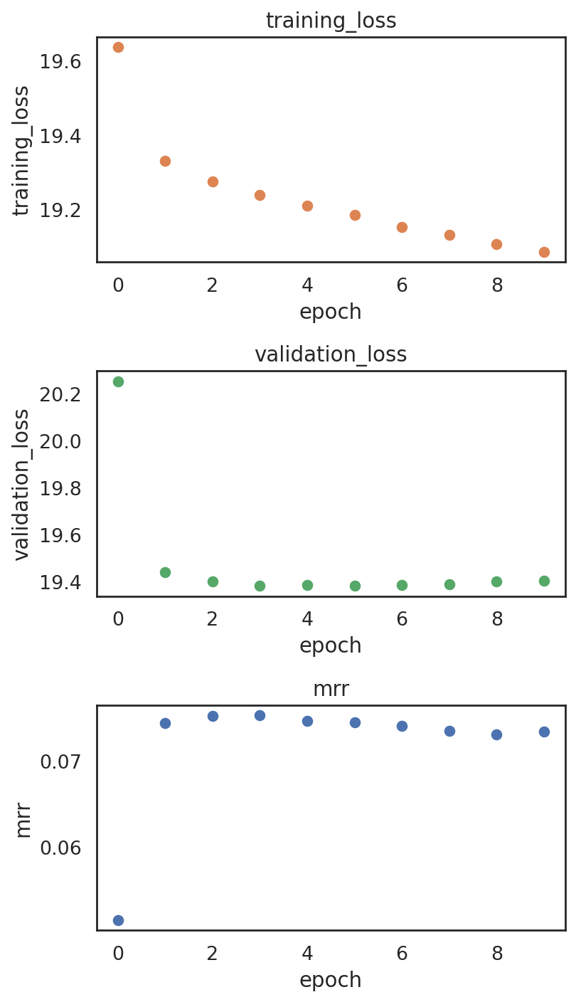
Plotting training metrics to monitor overfitting and evaluate the final model. Ideally, after a certain number of epochs, the metric curve should stabilize and remain steady.
By default, training loss (lower is better) along with validation loss (lower is better) and MRR (higher is better) are shown.
[15]:
si.pl.pbg_metrics(fig_ncol=1)
[ ]:
If further parameter tuning is required, generating new embeddings using updated parameters while training on the same graph can be achieved by updating the output variable, e.g.,
si.tl.pbg_train(pbg_params = dict_config, auto_wd=True, save_wd=True, output="model2")
The new result will be stored in ./result_simba_rnaseq/pbg/graph0/model2.
[ ]:
If needed, the PBG training parameters can be updated using the following function, once the training parameters have been finalized:
si.settings.set_pbg_params(dict_config)
If no parameters are specified, si.settings.set_pbg_params() will reset PBG training parameters to the step before graph generation.
[ ]:
To load the trained result, the following steps can be taken:
By default, it uses the current training result stored in .setting.pbg_params
# load back 'graph0'
si.load_graph_stats()
# load back 'model' that was trained on 'graph0'
si.load_pbg_config()
Users can also specify different paths, e.g.,
# load back 'graph1'
si.load_graph_stats(path='./result_simba_rnaseq/pbg/graph1/')
# load back 'model2' that was trained on 'graph1'
si.load_pbg_config(path='./result_simba_rnaseq/pbg/graph1/model2/')
[ ]:
Post-training analysis
[20]:
# read in entity embeddings obtained from pbg training.
dict_adata = si.read_embedding()
dict_adata
[20]:
{'C': AnnData object with n_obs × n_vars = 2700 × 50,
 'G': AnnData object with n_obs × n_vars = 13714 × 50}
[21]:
adata_C = dict_adata['C']  # embeddings of cells
adata_G = dict_adata['G']  # embeddings of genes
[ ]:
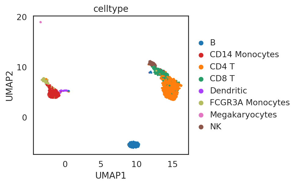
visualize embeddings of cells
[22]:
## Add annotation of celltypes (optional)
adata_C.obs['celltype'] = adata_CG[adata_C.obs_names,:].obs['celltype'].copy()
adata_C
[22]:
AnnData object with n_obs × n_vars = 2700 × 50
    obs: 'celltype'
[23]:
palette_celltype={'B':'#1f77b4',
                  'CD4 T':'#ff7f0e',
                  'CD8 T':'#279e68',
                  'Dendritic':"#aa40fc",
                  'CD14 Monocytes':'#d62728',
                  'FCGR3A Monocytes':'#b5bd61',
                  'Megakaryocytes':'#e377c2',
                  'NK':'#8c564b'}
[24]:
si.tl.umap(adata_C,n_neighbors=15,n_components=2)
si.pl.umap(adata_C,color=['celltype'],
           dict_palette={'celltype': palette_celltype},
           fig_size=(6,4),
           drawing_order='random')
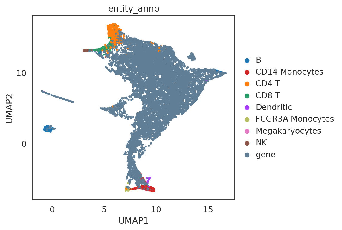
[ ]:
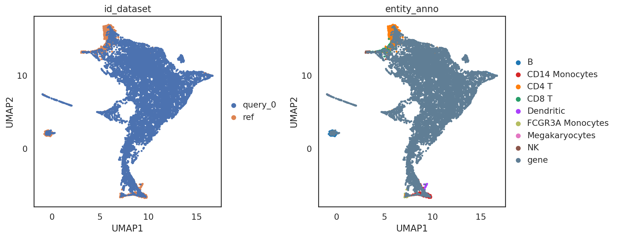
visualize embeddings of cells and all genes
[25]:
# embed cells and genes into the same space
adata_all = si.tl.embed(adata_ref=adata_C,list_adata_query=[adata_G])
adata_all.obs.head()
Performing softmax transformation for query data 0;
[25]:
| celltype | id_dataset | |
|---|---|---|
| GACTCCTGTTGGTG-1 | CD14 Monocytes | ref |
| TCTAACACCAGTTG-1 | NK | ref |
| GAAACCTGTGCTAG-1 | CD4 T | ref |
| CATTACACCAACTG-1 | NK | ref |
| ACTCAGGATTCGTT-1 | CD14 Monocytes | ref |
[26]:
## add annotations of cells and genes
adata_all.obs['entity_anno'] = ""
adata_all.obs.loc[adata_C.obs_names, 'entity_anno'] = adata_all.obs.loc[adata_C.obs_names, 'celltype']
adata_all.obs.loc[adata_G.obs_names, 'entity_anno'] = 'gene'
adata_all.obs.head()
[26]:
| celltype | id_dataset | entity_anno | |
|---|---|---|---|
| GACTCCTGTTGGTG-1 | CD14 Monocytes | ref | CD14 Monocytes |
| TCTAACACCAGTTG-1 | NK | ref | NK |
| GAAACCTGTGCTAG-1 | CD4 T | ref | CD4 T |
| CATTACACCAACTG-1 | NK | ref | NK |
| ACTCAGGATTCGTT-1 | CD14 Monocytes | ref | CD14 Monocytes |
[27]:
palette_entity_anno = palette_celltype.copy()
palette_entity_anno['gene'] = "#607e95"
[28]:
si.tl.umap(adata_all,n_neighbors=15,n_components=2)
si.pl.umap(adata_all,color=['id_dataset','entity_anno'],
           dict_palette={'entity_anno': palette_entity_anno},
           drawing_order='original',
           fig_size=(6,5))
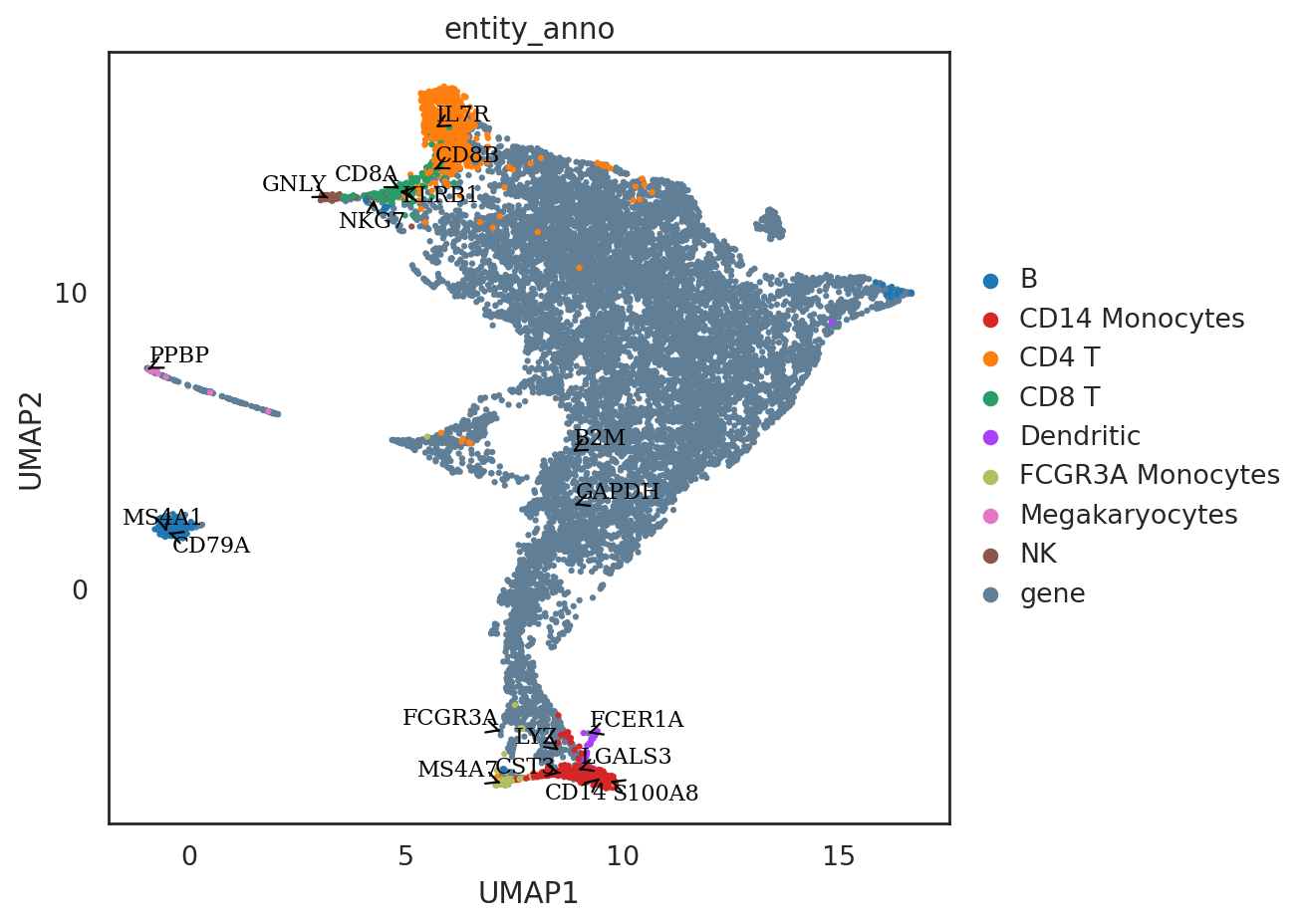
[29]:
# highlight some marker genes in the co-embedding space
marker_genes = ['IL7R', 'CD79A', 'MS4A1', 'CD8A', 'CD8B', 'LYZ', 'CD14',
                'LGALS3', 'S100A8', 'GNLY', 'NKG7', 'KLRB1',
                'FCGR3A', 'MS4A7', 'FCER1A', 'CST3', 'PPBP']
si.pl.umap(adata_all[::-1,],color=['entity_anno'],dict_palette={'entity_anno': palette_entity_anno},
           drawing_order='original',
           texts=marker_genes + ['GAPDH', 'B2M'],
           show_texts=True,
           fig_size=(8,6))
[ ]:
We can also visualize only partial genes (e.g., variable genes) instead of all genes by following the steps below:
# obtain variable genes
si.pp.select_variable_genes(adata_CG, n_top_genes=3000)
var_genes = adata_CG.var_names[adata_CG.var['highly_variable']].tolist()
# obtain SIMBA embeddings of cells and variable genes
adata_all2 = adata_all[list(adata_C.obs_names) + var_genes,].copy()
# visualize them using UMAP
si.tl.umap(adata_all2,n_neighbors=15,n_components=2)
si.pl.umap(adata_all2,color=['entity_anno'],
           dict_palette={'entity_anno': palette_entity_anno},
           drawing_order='original',
           fig_size=(6,5))
[ ]:
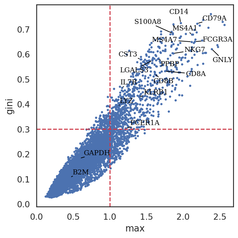
clustering-free marker discovery
compute SIMBA metrics including max value, Gini index, standard deviation, and entropy, to assess cell-type specificity of genes:
max: a higher value indicates higher cell-type specificity
gini: a higher value indicates higher cell-type specificity
std: a higher value indicates higher cell-type specificity
entropy: a lower value indicates higher cell-type specificity
[30]:
adata_cmp = si.tl.compare_entities(adata_ref=adata_C, adata_query=adata_G)
adata_cmp
[30]:
AnnData object with n_obs × n_vars = 2700 × 13714
    obs: 'celltype'
    var: 'max', 'std', 'gini', 'entropy'
    layers: 'norm', 'softmax'
[31]:
# genes can be ranked based on either one or multiple metrics
adata_cmp.var.head()
[31]:
| max | std | gini | entropy | |
|---|---|---|---|---|
| YIPF5 | 0.540598 | 0.229048 | 0.129493 | 7.874485 |
| ZDHHC7 | 0.652473 | 0.322003 | 0.184971 | 7.846139 |
| PSAP | 1.165987 | 0.656630 | 0.384751 | 7.636724 |
| ARL4C | 1.068365 | 0.625148 | 0.327085 | 7.730876 |
| MYO19 | 0.325210 | 0.109136 | 0.060507 | 7.894761 |
[32]:
# SIMBA metrics can be visualized using the following function:
si.pl.entity_metrics(adata_cmp,
                     x='max',
                     y='gini',
                     show_contour=False,
                     texts=marker_genes + ['GAPDH', 'B2M'],
                     show_texts=True,
                     show_cutoff=True,
                     size=5,
                     text_expand=(1.3,1.5),
                     cutoff_x=1.,
                     cutoff_y=0.3,
                     save_fig=False)
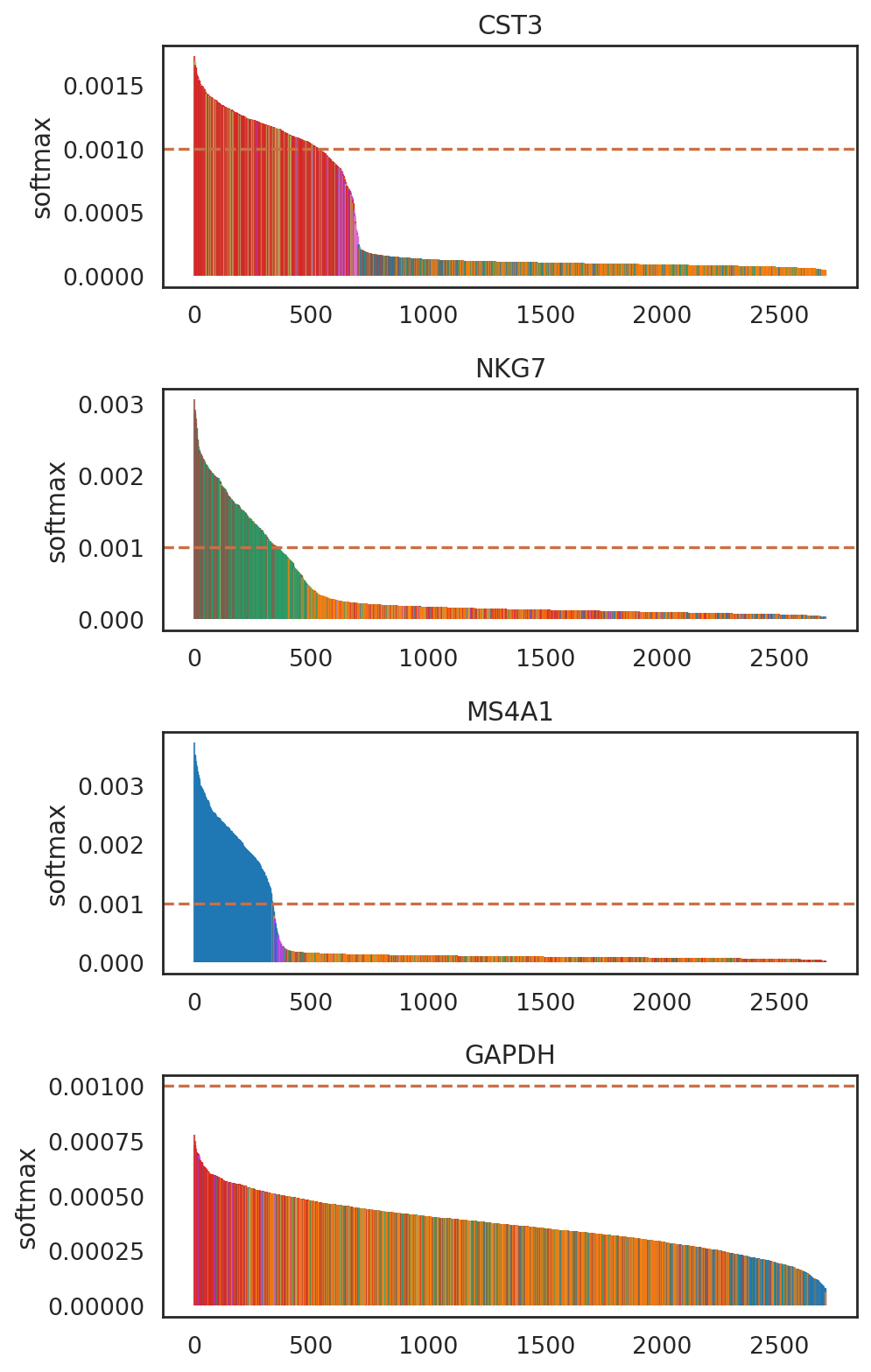
[ ]:
SIMBA barcode plot
SIMBA barcode plots visualize feature-cell probability based on edge confidence: - Imbalance indicates cell-type specificity - uniform distribution suggests non-specificity.
SIMBA barcode plots
[33]:
# add annoations of cells
adata_cmp.obs['celltype'] = adata_CG.obs.loc[adata_cmp.obs_names,'celltype']
list_genes = ['CST3', 'NKG7', 'MS4A1', 'GAPDH']
si.pl.entity_barcode(adata_cmp,
                     layer='softmax',
                     entities=list_genes,
                     anno_ref='celltype',
                     show_cutoff=True,
                     cutoff=0.001,
                     palette=palette_celltype,
                     fig_size=(6, 2.5),
                     save_fig=False)
[ ]:
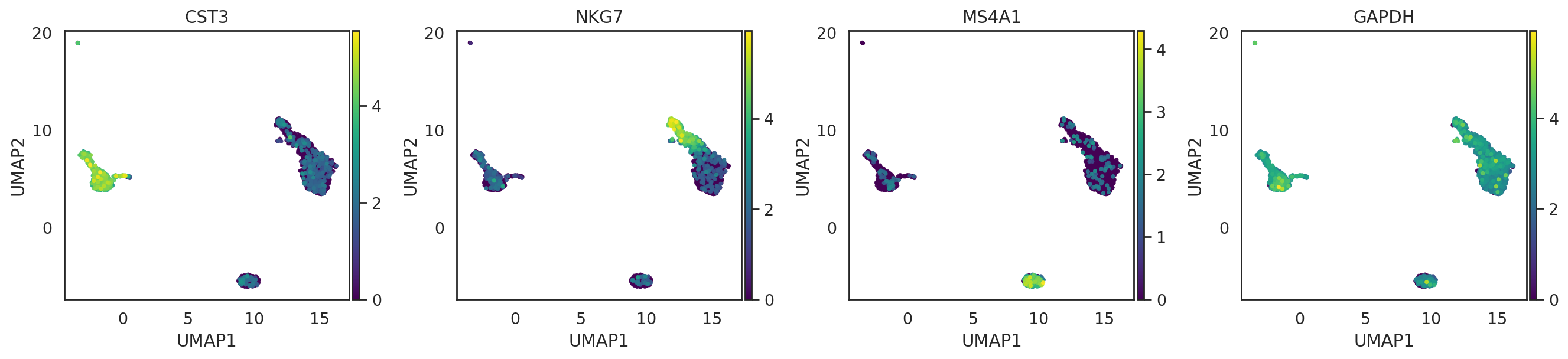
[35]:
# The same list of genes can also be visualized on UMAP to confirm their cell type specificity
adata_CG.obsm['X_umap'] = adata_C[adata_CG.obs_names,].obsm['X_umap'].copy()
si.pl.umap(adata_CG,
           color=['CST3', 'NKG7', 'MS4A1', 'GAPDH'],
           drawing_order='sorted',
           size=5,
           alpha=0.9,
           fig_ncol=4,
           fig_size=(4,4),
           save_fig=False)
[ ]:
Queries of entities in SIMBA space
The SIMBA embedding space, with cells and features, serves as an informative entity database. Queries can be performed on the “SIMBA database” by examining neighboring entities at the individual-cell or individual-feature level.
For example, - the query for a cell’s neighboring features can be used to identify marker features (e.g., marker genes) at the individual-cell level. - the query for features’ neighboring cells can be used to annotate cells.
[36]:
# First, we visualize the SIMBA co-embedding space, which serves as a database of entities including both cells and features (e.g., genes) and also where queries of entities will be performed
si.pl.umap(adata_all,
           color=['entity_anno'],dict_palette={'entity_anno': palette_entity_anno},
           drawing_order='random',
           show_texts=False,
           fig_size=(7,5))
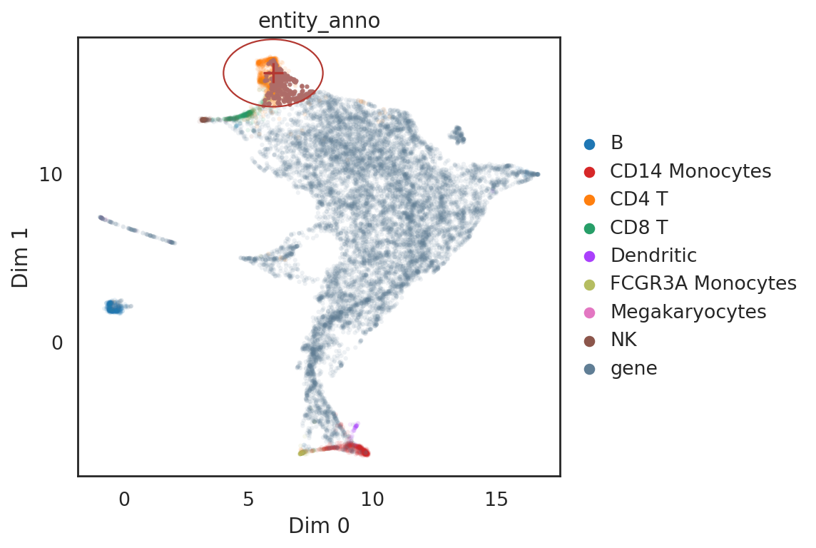
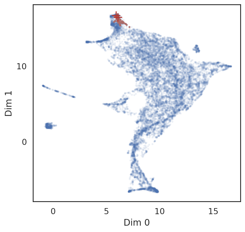
[37]:
# find neighbor genes around the location [6, 16] on UMAP
query_result = si.tl.query(adata_all,
                           pin=[6,16],
                           obsm='X_umap',
                           use_radius=True,r=2,
                           anno_filter='entity_anno',
                           filters=['gene'])
print(query_result.shape)
query_result.head()
(247, 5)
[37]:
| celltype | id_dataset | entity_anno | distance | query | |
|---|---|---|---|---|---|
| AC013264.2 | nan | query_0 | gene | 0.001936 | 0 |
| PCSK1N | nan | query_0 | gene | 0.069059 | 0 |
| TCEA3 | nan | query_0 | gene | 0.082872 | 0 |
| CD27 | nan | query_0 | gene | 0.091110 | 0 |
| RP11-18H21.1 | nan | query_0 | gene | 0.105336 | 0 |
[38]:
# show locations of pin point and its neighbor genes
si.pl.query(adata_all,
            show_texts=False,
            color=['entity_anno'], dict_palette={'entity_anno': palette_entity_anno},
            alpha=0.9,
            alpha_bg=0.1,
            fig_size=(7,5))
[ ]:
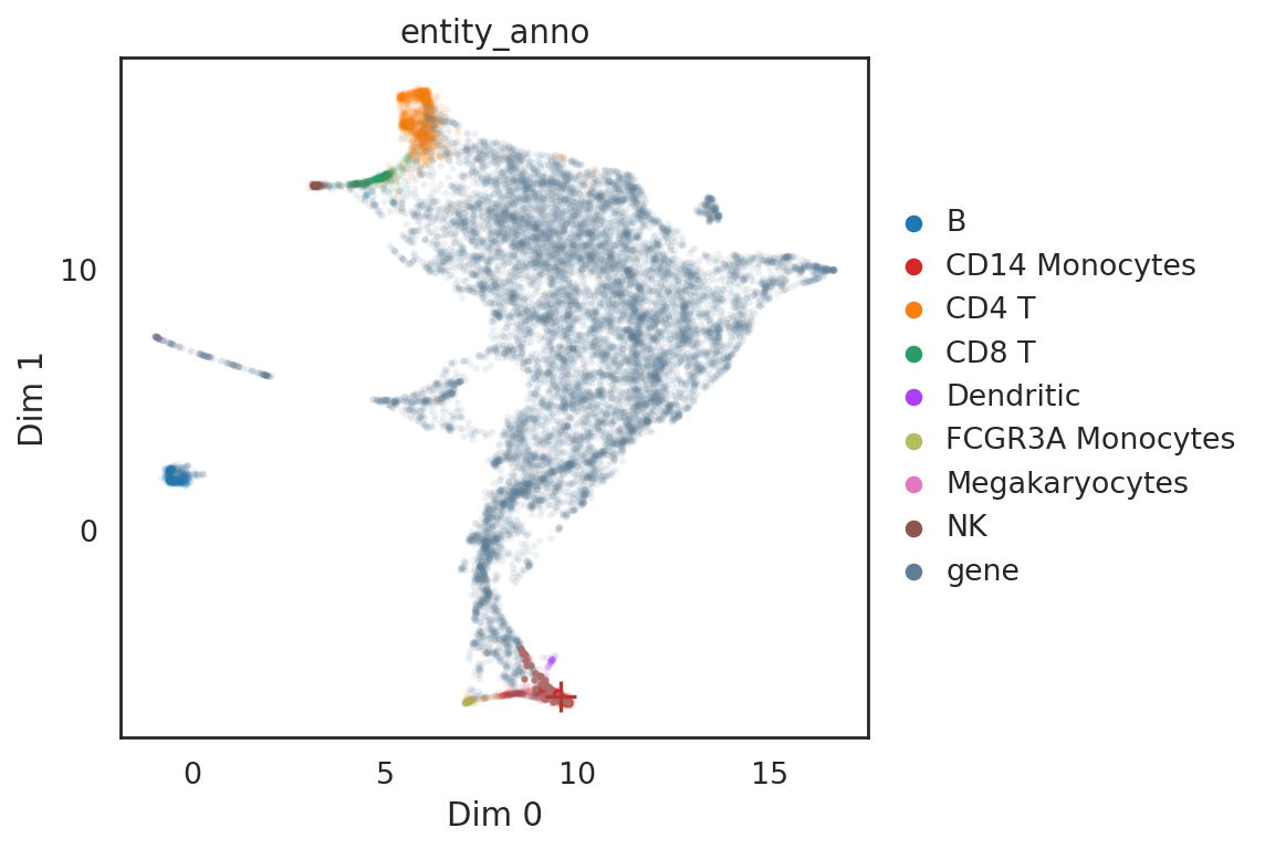
[39]:
# find top 50 neighbor genes around cell "ACTCAGGATTCGTT-1" (CD14 Monocytes) in SIMBA space
query_result = si.tl.query(adata_all,
                           entity=['ACTCAGGATTCGTT-1'],
                           obsm=None,
                           use_radius=False,
                           k=50,
                           anno_filter='entity_anno',
                           filters=['gene'])
print(query_result.shape)
query_result.head()
(50, 5)
[39]:
| celltype | id_dataset | entity_anno | distance | query | |
|---|---|---|---|---|---|
| JUND | nan | query_0 | gene | 1.719076 | ACTCAGGATTCGTT-1 |
| CLEC4E | nan | query_0 | gene | 1.728315 | ACTCAGGATTCGTT-1 |
| PTPRE | nan | query_0 | gene | 1.729887 | ACTCAGGATTCGTT-1 |
| QPCT | nan | query_0 | gene | 1.731332 | ACTCAGGATTCGTT-1 |
| NUP214 | nan | query_0 | gene | 1.733139 | ACTCAGGATTCGTT-1 |
[40]:
# show locations of entity and its neighbor genes
si.pl.query(adata_all,
            obsm='X_umap',
            color=['entity_anno'], dict_palette={'entity_anno': palette_entity_anno},
            alpha=0.9,
            alpha_bg=0.1,
            fig_size=(7,5))
[ ]:
[41]:
# find top 50 neighbor genes for multiples cells in SIMBA space
query_result = si.tl.query(adata_all,entity=['GATGCCCTCTCATT-1', 'CTGAAGTGGCTATG-1'],
                           obsm=None,
                           use_radius=False,
                           k=50,
                           anno_filter='entity_anno',
                           filters=['gene'],
                           )
print(query_result.shape)
query_result.head()
(100, 5)
[41]:
| celltype | id_dataset | entity_anno | distance | query | |
|---|---|---|---|---|---|
| LINC00176 | nan | query_0 | gene | 1.020504 | CTGAAGTGGCTATG-1 |
| CCR7 | nan | query_0 | gene | 1.021033 | CTGAAGTGGCTATG-1 |
| FHIT | nan | query_0 | gene | 1.021289 | CTGAAGTGGCTATG-1 |
| LDLRAP1 | nan | query_0 | gene | 1.040456 | GATGCCCTCTCATT-1 |
| TSHZ2 | nan | query_0 | gene | 1.047881 | GATGCCCTCTCATT-1 |
[42]:
# show locations of entities and their neighbor genes
si.pl.query(adata_all,
            obsm='X_umap',
            alpha=0.9,
            alpha_bg=0.1,
            fig_size=(5,5))
[ ]:
[43]:
# find neighbor entities (both cells and genes) of a given gene on UMAP
query_result = si.tl.query(adata_all,
                           entity=['CD79A'],
                           obsm='X_umap',
                           use_radius=False,
                           k=50
                           )
print(query_result.shape)
query_result.iloc[:10,]
(50, 5)
[43]:
| celltype | id_dataset | entity_anno | distance | query | |
|---|---|---|---|---|---|
| CD79A | nan | query_0 | gene | 0.000000 | CD79A |
| CD19 | nan | query_0 | gene | 0.013946 | CD79A |
| TGGATGTGACCTAG-1 | B | ref | B | 0.014974 | CD79A |
| ACAAGAGAGTTGAC-1 | B | ref | B | 0.016267 | CD79A |
| TACATCACGCTAAC-1 | B | ref | B | 0.022173 | CD79A |
| TTATCCGACTAGTG-1 | B | ref | B | 0.024351 | CD79A |
| GGAACTTGGGTAGG-1 | B | ref | B | 0.025603 | CD79A |
| TGCGTAGACGGGAA-1 | B | ref | B | 0.027751 | CD79A |
| TAACTCACGTACAC-1 | B | ref | B | 0.028147 | CD79A |
| GATTGGACTTTCGT-1 | B | ref | B | 0.029059 | CD79A |
[44]:
si.pl.query(adata_all,
            obsm='X_umap',
            color=['entity_anno'], dict_palette={'entity_anno': palette_entity_anno},
            show_texts=False,
            alpha=0.9,
            alpha_bg=0.1,
            fig_size=(7,5))

[ ]:
save results
[45]:
adata_CG.write(os.path.join(workdir, 'adata_CG.h5ad'))
adata_C.write(os.path.join(workdir, 'adata_C.h5ad'))
adata_G.write(os.path.join(workdir, 'adata_G.h5ad'))
adata_all.write(os.path.join(workdir, 'adata_all.h5ad'))
adata_cmp.write(os.path.join(workdir, 'adata_cmp.h5ad'))
[ ]:
Read back anndata objects
adata_CG = si.read_h5ad(os.path.join(workdir, 'adata_CG.h5ad'))
adata_C = si.read_h5ad(os.path.join(workdir, 'adata_C.h5ad'))
adata_G = si.read_h5ad(os.path.join(workdir, 'adata_G.h5ad'))
adata_all = si.read_h5ad(os.path.join(workdir, 'adata_all.h5ad'))
adata_cmp = si.read_h5ad(os.path.join(workdir, 'adata_cmp.h5ad'))